Nov 23 2009
Alarmists Hide Truth About (Lack Of) Global Warming
Notice: Sorry folks, going back and cleaning up errors, trying to use English as my language, etc. You might find changes from the first read.
Update: Could the CRU data plots I discuss below be the raw data that shows cooling since 1960 that was noted as a ‘trick’ in emails and CRU source code? – end update
I have not had to work this hard on a post for quite a while, but the topic is – after all – the total annihilation of the Earth by man-made CO2. So I have set aside some work and free time to investigate some critical data that shows, without much doubt, that man-made global warming is a con, a false alarm created by shoddy statistics and faux science. The emails and data are conclusive in demonstrating a  pattern of cover up and misinformation in this matter by CRU and others (especially if they were to be presented to a grand jury for possible indictment).
I will say this up front: some alarmist may have been overcome by self obsession over becoming apparent heros to planet Earth and all humankind. Not pretty, but understandable. But others are strictly in it for the power and the money, and I will let history sort who falls were. I will also say this, the person who hacked the Hadley Climate Research Unit (CRU) did the world a huge favor by exposing the real data behind all the global warming false alarms.
I am going to focus this post on two key documents that became public with the recent whistle blowing at CRU. The first document concerns the accuracy of the land based temperature measurements, which make up the core of the climate alarmists claims about warming. When we look at the CRU error budget and error margins we find a glimmer of reality setting in, in that there is no way to detect the claimed warming trend with the claimed accuracy.
The second document contains 155 graphs showing the raw global temperature measurements and ‘trends’ for every country from 1900 though today. It contains two version of the CRU ‘processing’ – one from 2005 and one from 2008. What is just amazing from this ‘raw’ data is the realization that many areas of the Earth are not showing a huge upswing in temperature. The raw data paints a completely different picture than the final ‘results’ we see in Al Gore’s charts. And we also get a glimpse at the ‘1940’s blip’ that was the subject of so many emails.
This post will review my analysis to date on the Americas, which is the section of the data I have had a chance to review and assess. I plan to do a region by region analysis over the coming weeks.
Before we dive into CRU data we need to step back and understand the concept of ‘accuracy’ in scientific measurements. One rule of reality is you cannot process data (run statistics) to create more accuracy than originallly captured in the raw data. If you measure something in meters or yards, no amount of statistical analysis can increase your accuracy to inches or centimeters. The best way to explain this is to use the commonly understood accuracy that is related to pictures – a.k.a. resolution.
Resolution = focus = ability to detect details. My biggest problem with (and challenge to) the alarmists’ global warming data is their ridiculous accuracy claims. Even if you can make the case for modern day accuracy (which has not been proven), you cannot apply that same accuracy back over a century of technological advances. As you go back in time the error bars grow immensely as the accuracy degrades.
To illustrate this I have two ‘global’ images of Mars taken from Earth about 50 years apart. Both were taken by state of the art systems of their time. First is an image of Mars from 1956 taken at the Mt Wilson Observatory (click to enlarge, but it doesn’t help much):
Here is the second, modern image (click to enlarge):
This second image was taken in 2001 from the Hubble Space Telescope. I had to lower the resolution of the second image to avoid long page loading delays, you can download the fully detailed image at the link. Even with this reduction in resolution it is not even a fair fight between 1950’s and the 2000’s.
This is a very reasonable and clear comparison of the technological capabilities of humanity between today and over half a century ago. These images represent state of the art accuracy for their days on global scales, and both were taken from basically the same distance. If you want to go back to the origin of the global temperature record (late 1800’s), you have to go back to the drawings (and wrong conclusions) of Percival Lowell. In other words accuracy degrades as we use older and older data.
There is no amount of statistical processing that can be done on the 1956 mars image data to make it as crisp and clear as the 2001 image data. When you think back to 1880, when the global temperature record began, you realize the error bars for that period (pre-electricity, etc) have to be huge – yet when it comes to global warming they apparently (and without any proof) are not!
Let’s review the current global warming claims on temperature changes and accuracy, which are best illustrated with this graph from NCDC (click to enlarge):

The diagram claims the modern ‘global temp index’ is accurate to +/- 0.05°C 0.5°C, and only grows to +/-  0.15°C 1.5°C when we travel back in time to 1880. This is just plain bogus. Before I explain why I also want to note the size of the so-called temperature anomaly depicted on this graph. It shows a -0.3°C (circa 1910) to +0.5°C (circa 2000) change over the period. Therefore the error in temp data cannot exceed 0.5°C or else all these global temp indexes are statistically equal (i.e., no warming).
So what is the actual error that goes into these global indexes? You don’t have to be a rocket scientist to figure out the sources of error (though it does help). What we have to do is define the error budget (each step that introduces new error in the global index data point). I can see this going through at least 6 phases that begin at taking a temperature reading on the surface of planet Earth:
- 1st is the measurement itself, including the accuracy of the measurement system (both for time and temp).
- 2nd is the local extrapolation of this point temperature to the surrounding area to create regional temp  (or grid in the parlance of the scientists).
- 3rd is the averaging of day and night measurements for a grid to cover a monthly period.
- 4th is the averaging of a series of local monthly estimates into a country-wide estimate for the month.
- 5th is averaging the monthly data into seasonal data points (CRU defines 4 seasons in its data) for each country
- 6th is computing a Southern Hemisphere, Northern Hemisphere and Global index from the annual seasonal-country data.
There are more sources of error (such as combing land and sea based measurements, satellite measurements, proxies, etc), but these 6 steps will suffice for now.
The first CRU document I noted above contains the CRU claims for errors through step 1- 3, and is quite stunning. Here is their unsubstantiated claim for step one – the measurement:
- Uncertainties in the station data:
- Measurement error: following [5] we estimate this as 0.04C on monthly average temperatures.
- Uncertainty in homogenisation corrections: we are estimating this by examining records of corrections performed at CRU, and by examining differences between corrected and uncorrected data provided by the Austrian and Canadian national met. services.
- Uncertainty in the climatologies: this is only important where station data is incomplete over the climatology period; we are estimating it by exploring the effect of removing data from stations with complete coverage.
Emphasis mine. I might buy the idea a single thermometer measurement today can be accurate to +/- 0.04°C, but I am not buying it over a region or over a month – and I am not buying it back in time. And here are two clear reasons why.
Addendum: But even more importantly, the station temperature which supposedly is accurate to 0.04°C cannot go through 6 plus steps of massaging and turn out a global index with an error of 0.05°C! That is impossible. – end addendum
Time & Accuracy of Measurement: To create a daytime and nighttime temperature record for a ‘station’ you need to take the temperatures at the exact same time relative to the UTC (the world wide time reference also known as Greenwich Time) each day. If you are off in time you throw all your data off. In the modern era that is made possible because of the GPS Satellite network, which can lock any computer any where on the globe to UTC with microsecond or better accuracy. Prior to GPS there was no cheap and effective way to link stations to a common time reference. As we go back in time the local accuracy of time degrades incredibly fast. Back in the 1960’s a local clock could be off by many seconds unless it was linked to a very expensive network of atomic clocks (not available to very many countries at that time and not cost effective for weather stations even here in the US). This loss of time accuracy, in my mind, easily degrades temps in the 1960’s to at least 0.5°C. And this  is before we take into account the thermometers’ accuracies. In 1880 I doubt all of the temp records were even accurate to+/- 0.25°C (a quarter of a degree). Combining the accuracy limitations on the devices and the timing of the measurement you are already well outside the claimed accuracy.
Regional Temp Extrapolation: Go to your weather channel TV station or website and look at the temperature variability in your area. Temps can be off by 2-5° if there is a massive front coming through. And since fronts come through any time of day you cannot extrapolate a local temp value more than a couple of miles before the potential errors become huge. Even if you know the time, without knowing the local weather there is no way to claim a single point represents any significantly sized region.  And once you expand this from a local region to an entire country you can see how the errors have to be in the +/- 1° C range even for today’s technology. These people claiming global warming exists at 0.8°C level with an accuracy of 0.05°C just don’t have the detailed data to back up their claims.
Anyway, I don’t need to do a lot on the error budget (that is for the alarmists to prove and defend). What surprised me was the one CRU document where CRU proves there is no demonstrable global warming (even by their own ridiculously optimistic assessment). Check out this graph  from their report (click to enlarge):
The title of this graph indicates this is the CRU computed sampling (measurement) error in C for 1969. Note how large these sampling errors are. They start at 0.5°C, which is the mark where any indication of global warming is just statistical noise and not reality. Most of the data is in the +/- 1°C range, which means any attempt to claim a global increase below this threshold is mathematically false. Imagine the noise in the 1880 data! You cannot create detail (resolution) below what your sensor system can measure. CRU has proven my point already – they do not have the temperature data to detect a 0.8°C global warming trend since 1960, let alone 1880.
Now let’s get back to the shape of that NCDC chart above and how it seems to show a slowly but steadily rising global temperature index from 1900-2008. Would anybody be surprised to find that the CRU land temp data just made public definitely DOES NOT show this trend?
Let me show you some interesting records from the 2nd CRU file I mentioned above. Thankfully I don’t need to dive in deep because the first set of data (Argentina) is sufficient to illustrate the apparent misinformation coming from the alarmists, and possibly how it is done. Here are the CRU records for Argentina (click to enlarge a bit, but go to the doc link to really zoom in):
Does anyone see a slowly rising warming trend? No, we don’t. What we see is a flat oscillating temperature with varying highs and lows, but the current time is not a lot warmer than any other time period. In fact, if you look at most of the country graphs from South America they show the same thing – no warming.
Some guidance on these charts are in order. First there are 4 graphs for the 4 seasons CRU uses to derive an annual global index (the NCDC level chart). MAM in the upper left panel stands for March-April-May, the next panel is June-July-August (JJA), etc. The purple data is the 2008 version of the data series, and the black line is the 2005. The dashed horizontal line is the mean for that country for that season: red is for the CRU 2008 version and black is for CRU 2005.
What is most troubling mathematically is the trend line, so let me blow one of these up for a closer look, but this time I am going to chose Chile MAM (for reasons which will become very apparent):
Again, we see no real warming in this season for Chile, but what I highlighted in the green box is the now infamous ‘1940’s blip’ (which seemed to be the subject of much CRU email has how best to ‘hide’ it from the world). Addendum: This data shows the 1940’s a good 0.5°C warmer than today. – end addendum
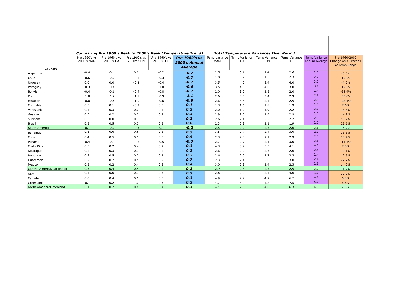
All across South America you see two things – no global warming and the 1940’s blip showing it cooler now than in the 1940’s. It shows up across the continent (and the world). When you move to Central America you see a 1950’s blip on top of slight global warming (+0.3°C on average). Up in North America you see mostly flat temps again with a slight uptick (+0.3°C). South America actually COOLED by an average of -0.2°C over this period.
I derived a cooling or warming factor by identifying any peak in the trend line that existed prior to 1960 and comparing it to trend line point in the 2000 era. Correction: Using this method I could see if the 2000 temps were unique, never before seen as claimed. For the MAM season in Chile this factor is -0.5 since the 1940’s peak was 0.5°C below the current period. – end correction.
If we recall the CRU claims its best margin of error is +/1 °C we can conclude that mathematically there has been no global warming detected in the CRU data (at least in the Americas, which is all I had the time to analyze in detail).
Since I had to do this by eyeballs the numbers are not precise, but the trends are clear. You look at a region and you see the same trends showing up over and over again. My data on the Americas can be found here, where the left hand data set is the difference in peak high temps between the pre 1960 era and the 2000. It clearly illustrates there is no significant warming in the trend lines for the countries of the Americas – especially in South America were global cooling is happening, which probably explains why the Antarctic Ice Extend has been growing for decades.
But what really bugs me is the way CRU suppresses reality in this processing. If you look at any one graph you can easily see that the ‘raw’ temperature range for that country is quite broad (even though this is processed from daily stations to create yearly data). You can see the ‘raw’ data has quite a large variability that the trend line mutes. In the Chile MAM panel there is a measurement range of 1.8°C, while the peak-to-peak delta in the trend is only -0.6°C.
What happens when you use the smoothed trend line is you DECREASE accuracy be removing the real life fluctuations. We are losing details in this smoothing process, the picture has become very fuzzy to detail. If you think of the error budget above as steps which remove or hide reality behind statistical noise, you can see why the NCDC chart looks nothing like the CRU charts. CRU and NCDC has ‘smoothed’ away reality to the point it is unreal. Toss in a few well selected proxies and you get man-made global warming graphs.
Here are some more examples of countries without measurable global warming (beyond the CRU stated margin of error): Bolivia, Greenland and Peru. There are many, many more such examples.
Again referring to my file of analysis on the Americas, I created a second data set from  the temperature ranges in the CRU panels, and then computed the peak-to-peak change as a percentage of that range (far right, orange column). I wanted to see if the peak-to-peak changes since prior to 1960 were a major fraction of the overall natural temperature variability. They of course were not. None of the changes appear out of the normal variation in temperature, variation lost in the trend lines.
What I did see were stronger indications of warming near the equator than nearer the poles. This could indicate the warming IS in fact caused by changes in solar radiation output, not man made CO2. I also find it interesting that the 1940’s temperature blip had seemingly moved to the equatorial region by the 1950’s and was creating a smaller blip there. There is a lot to learn from this data, and how it correlates to other events or conditions. But what is clear to me now is there was probably no way to create a hockey stick from this CRU data alone. Which is why we have things like bristle cones and magic larches in Russia to create the mirage of global warming.
What I see in this data is a valid and scientifically based argument AGAINST global warming. I detect only modest temp changes (well within the normal temperature variability) for Central America and Northern America, along with a clear cooling in South America. I can say with confidence that the supposed center of man-made CO2 production (America) is not experiencing runaway, CO2 induced warming (given the accuracy of the raw measurements and the ‘global index’).
The CRU data clearly indicates that. But I can also take the CRU emails and underscore how they represent a serious cover up, to wit this one email  the 1940’s blip:
Phil,
Here are some speculations on correcting SSTs to partly explain the 1940s warming blip.
If you look at the attached plot you will see that the land also shows the 1940s blip (as I’m sure you know).
So, if we could reduce the ocean blip by, say, 0.15 degC, then this would be significant for the global mean — but we’d still have to explain the land blip.
I’ve chosen 0.15 here deliberately. This still leaves an ocean blip, and i think one needs to have some form of ocean blip to explain the land blip (via either some common forcing, or ocean forcing land, or vice versa, or all of these). When you look at other blips, the land blips are 1.5 to 2 times (roughly) the ocean blips — higher sensitivity plus thermal inertia effects. My 0.15 adjustment leaves things consistent with this, so you can see where I am coming from.
Removing ENSO does not affect this.
It would be good to remove at least part of the 1940s blip, but we are still left with “why the blip”.
Let me go further. If you look at NH vs SH and the aerosol effect (qualitatively or with MAGICC) then with a reduced ocean blip we get continuous warming in the SH, and a cooling in the NH — just as one would expect with mainly NH aerosols.
This ‘inconvenient truth’ showed up in both the land and sea data. You can see it all over the world. And since it shows today not much different from then, it had to be deleted from history and CRU’s own data had to been kept under wraps.
I plan to do more analysis, completing my spread sheet for the entire 155 entries. This takes a lot of time, as you can imagine. But it is worth it to understand the scope of the misinformation and cover up that has gone on these many years by so called scientists.


[…] In my original post on these files I went into great detail on the aspect of measurement accuracy (or error bars) regarding alarmists claims. I will not repeat that information here, but I feel I am being generous giving the data a +/- 0.5°C margin of error on a trend line (which contains multiple layers of averaging error incorporated in it). Most of the CRU uncertainty data, as mapped on the globe, is above the 1°C uncertainty level. […]
[…] changes in uncertainty going back in time  – proof positive they screwed up their error budget. One of my first posts on Climategate was on errors in climate estimates over time, and I used space exploration again as […]
[…] Alarmists Hide Truth About (Lack Of) Global Warming […]